OpenAI has floated giving the US government a 5 percent ownership stake as a way of easing tensions with the Trump administration and blunting mounting public backlash against AI, according to the Financial Times.
CEO Sam Altman argued that giving the public a financial interest in the company would be the best way to share the upside of AI, the FT reported, citing two unnamed people familiar with the talks. He's said to have first pitched the idea to Trump early last year.
Altman reportedly suggested the 5 percent figure. Based on OpenAI's latest funding round, which ended with the company valued at $852 billion, that stake would be worth …
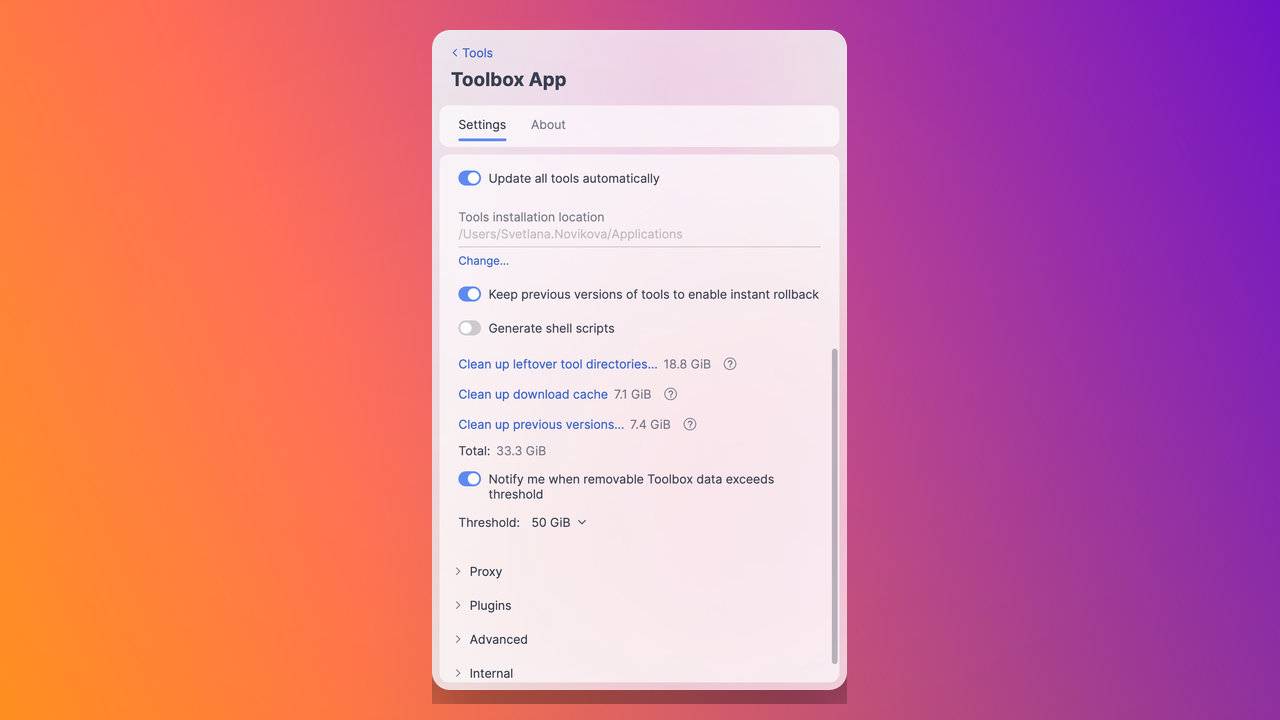
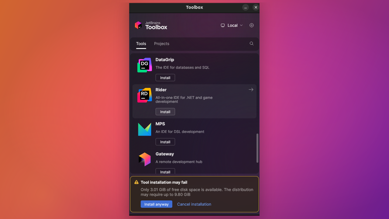
Toolbox App 3.6 gives you better control over local storage and makes Windows installation failures easier to diagnose.
Clean up removable Toolbox App data from Settings
The Toolbox App now shows how much removable data it can safely clean up, providing a breakdown for the download cache, previous versions, temporary leftovers, and leftover tool directories. Instead of inspecting cache folders manually, you can review and remove this data directly through Settings.
The app can suggest cleanup when it can help with a tool installation or update and you can set an optional cleanup reminder by choosing the amount of removable Toolbox App data that triggers a notification. See TBX-18085 for more details.
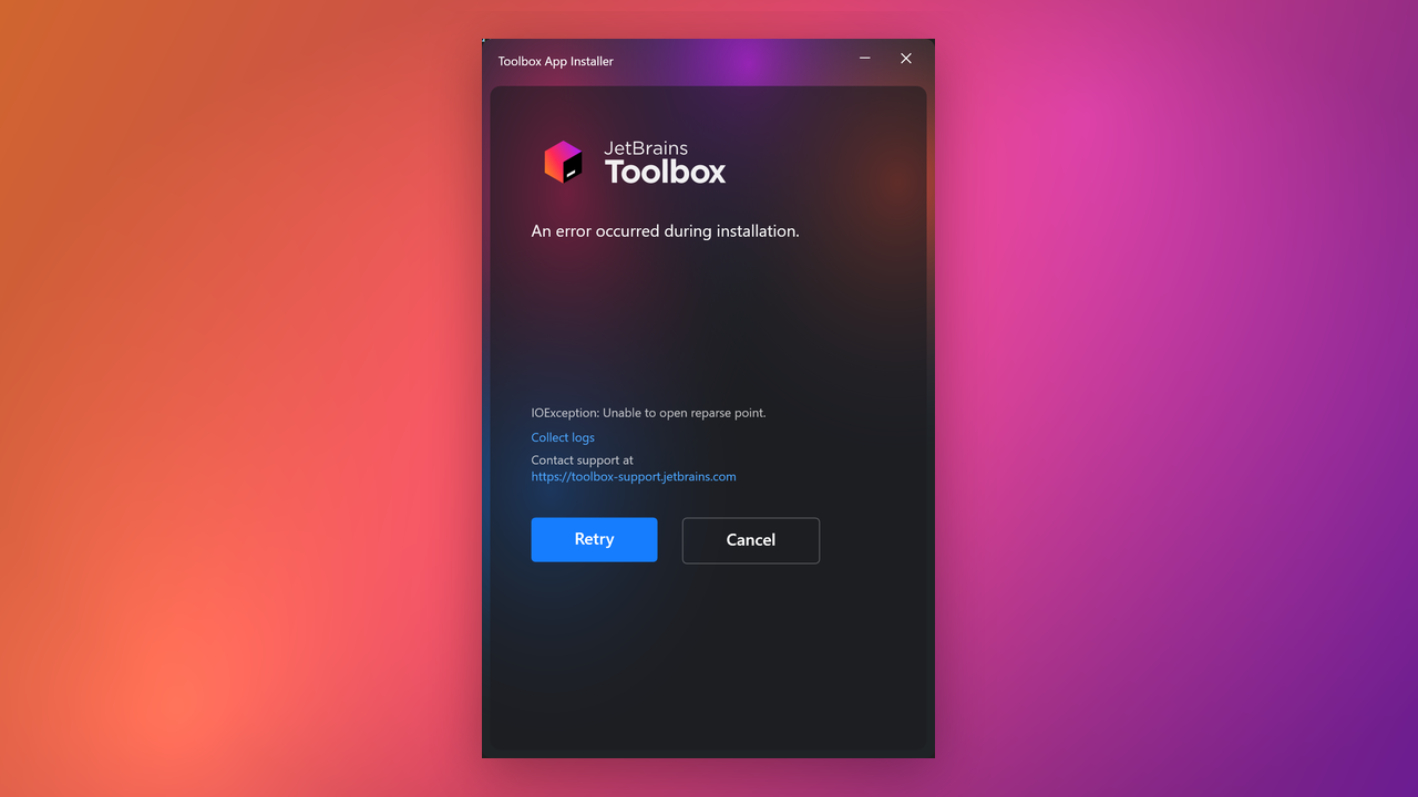
Clearer Windows installer diagnostics
When the Windows installer cannot write files, the Toolbox App now gives you more useful diagnostics instead of only showing a generic exception. The installer can point to the process blocking a file, show read-only file or folder problems, and help you collect logs to send to the support team. See TBX-18624 for more details.
No more CodeCanvas
CodeCanvas has been sunset and removed from the Toolbox App. See TBX-18717 for more details.
Several years ago, GitHub Security launched an initiative to assess and improve our overall secrets hygiene. As part of that effort, we piloted the Secret Scanning capability that was under development at the time. That’s when we found more than 20,000 secrets spread across our 15,000+ repositories.
The number was significantly higher than we anticipated, but it quickly became clear that success would depend on identifying which alerts represented real risk, assigning ownership, and remediating them safely. Nine months later, we reached zero open alerts.
New secret scanning customers often ask us: “How do you manage this internally? How did you actually clean up your existing secrets?”
Like many long-running software companies, GitHub’s approach to secrets management evolved over time. GitHub was founded in 2008, before today’s centralized vaults, automated secret scanning, and dedicated secrets-management platforms were common across the industry. As engineering practices matured and GitHub grew, we continued investing in stronger controls, better tooling, and systematic risk reduction for legacy patterns. This work reflects our ongoing commitment to improving security, reducing exposure, and ensuring our internal practices meet the same high standards we expect across the industry.
This blog post shares what worked for us during this effort, and highlights strategies you can apply to better protect your own secrets.
Cutting out the noise
The first thing we discovered was that the alert count was a bit misleading—i.e., 20,000 alerts did not mean 20,000 equally risky problems.
When we dug into the data, we discovered that just five repositories accounted for roughly 18,000 of those alerts, and every one of those secrets was inactive: test fixtures, deactivated credentials, and fake-but-valid-looking secrets used for testing. (We build secret scanning, so naturally we have repositories full of legitimate-looking secrets in tests.)
That left over 2,000 alerts that needed attention: potential live credentials and thousands of decisions about risk, rotation, and remediation.
Secrets don’t just live in code
Secret remediation touched more than source code. We found secrets in support tickets (customers occasionally include tokens), bug bounty reports (researchers disclose what they found with complete reproductions, including API requests with tokens used), incident notes, and wiki pages.
We partnered with customer support, security incident response, and our bug bounty program to develop shared playbooks. Across all these workflows, we had to ensure we weren’t creating new problems, like opening issues or pushing commits containing the very secrets we were trying to remediate.
Our phased approach
We were not going to close 20,000 alerts by asking a few security engineers to grind through them one by one. We treated it like any other operational backlog: stop new debt, then work down what already exists with a workflow that’s repeatable, measurable, and not dependent on one person’s institutional knowledge.
Phase 1: Enable everywhere, stop the accumulation
Before cleaning up existing secrets, we had to stop new ones from piling up.
We enabled secret scanning and push protection across all of our enterprises and organizations. Thanks to GitHub Advanced Security’s organization-level settings, this wasn’t a repository-by-repository slog across 15,000 repositories. We enforced the setting so individual repositories and teams could not quietly opt out.
Push protection blocked new secrets at the source. That kept the backlog from growing faster than we could burn it down.
Phase 2: Understand and triage
We broke down the 20,000+ alerts by repository, secret type, and age so we could separate noise from work.
When we dug in, we discovered that just five repositories accounted for roughly 18,000 of those alerts, and every one of those secrets was inactive: test fixtures, deactivated credentials, and fake-but-valid-looking secrets used for testing. (We build secret scanning, so naturally we have repositories full of legitimate-looking secrets in tests.)
For high-volume, low-risk alerts, we developed criteria for bulk closure. If a secret was in a dedicated test repository, had never been active, and matched a known test pattern, we could confidently mark it resolved. In a matter of days, we closed out roughly 18,000 alerts.
The hard questions
We had to make strategic decisions about how to remediate secrets. When a secret lives in an issue, do you edit the body (and potentially remove revision history), or preserve the audit trail? When a secret is committed to a repository, do you rewrite git history? Anyone who’s tried rewriting git history at scale knows what happens next: force-pushes break open pull requests, invalidate commit SHAs, and generally interrupt developers.
A common question was: “Can we just delete the repository if it’s no longer in use?” Our answer was generally no. A deleted repository takes its audit trail with it. If a secret in that repository was ever leaked or the repository was ever compromised, you lose the forensic record you’d need during incident response. Rotate the secret, archive the repository if appropriate, but keep the history.
Whenever possible, we rotate or revoke the exposed secret first. The harder question is whether the residual risk warrants rewriting git history, or whether a revoked secret in history can safely be left in place. These are the types of questions and decisions present with each alert that product security teams wrestle with.
Phase 3: Validate what’s actually live
A credential sitting in a repository might have been rotated years ago, or it might still unlock production systems. You can’t prioritize without knowing the difference.
At the time, secret scanning didn’t have native validity checking, so we built our own approach. The goal was narrow: determine whether a credential still worked and, when appropriate, collect enough metadata to route the alert or notify the right owner.
For example, for a GitHub token, a representative check could make a single authenticated request to a low-impact endpoint like GET /user:
response="$(
  curl -sS -w '\n%{http_code}' \
    -H "Authorization: Bearer $TOKEN" \
    -H "Accept: application/vnd.github+json" \
    -H "X-GitHub-Api-Version: 2022-11-28" \
    https://api.github.com/user
)"

status="${response##*$'\n'}"
body="${response%$'\n'*}"

case "$status" in
  200)
    login="$(jq -r '.login // empty' <<< "$body")"
    echo "token appears active for GitHub user: $login"
    ;;
  401)
    echo "token appears invalid or revoked"
    ;;
  403|429)
    echo "unable to determine validity; rate-limited or blocked"
    ;;
  *)
    echo "unable to determine validity: HTTP $status"
    ;;
esac
Remember, our goal was to answer the smallest useful set of questions: does this credential still work, and who needs to know about it? We treated ambiguous responses as inconclusive, and we avoided follow-on requests to repositories, organizations, or other private resources.
This required close partnership with our privacy and legal teams. Even a “read-only” validity check can have implications when you’re touching a credential you may not own.
As we worked through this manually, our product team built the solution natively, which made the remaining work much faster. Validity checking is now built into GitHub secret scanning.
Phase 4: Figure out who owns what
That cross-functional work also exposed an ownership problem: even after we knew a credential was active, we still had to figure out who could rotate it.
We partnered with customer support, security incident response, and our bug bounty program to develop shared playbooks for secrets reported outside of code. That included redacting secret values before routing work to teams, determining whether a credential belonged to GitHub or a customer, and notifying affected customers or researchers so they could rotate tokens under their control. Across all these workflows, we had to ensure we weren’t creating new problems, like opening issues or pushing commits containing the very secrets we were trying to remediate.
For GitHub-issued credentials like personal access tokens, we worked with our product team to surface secret metadata directly in the alert: who created the token, when, and what scopes it had. That meant we didn’t need to use the token itself to figure out who it belonged to.
For everything else, ownership was harder, and this exposed a deeper problem: not all repositories had clear owners.
Our internal engineering standards (the Engineering Fundamentals program) enforce durable ownership on services, and we maintain a mapping between services and repositories, but not all repositories map cleanly to a service. The pain we experienced led to a broader repository ownership initiative (using GitHub’s Custom Properties), plus a parallel effort to ensure all secrets in our credential manager have durable owners. You can’t rotate a secret if you can’t find the owner.
Phase 5: Manual triage for the long tail
Even with validation and metadata, a long tail of alerts required human judgment. For each one: what does this grant access to, has it been rotated, who owns the connected system, and what’s the remediation path?
For every alert we dismissed, we ensured an accurate disposition (e.g., revoked, used in test, false positive) was recorded, along with a comment containing relevant context, such as a link to a remediation issue or an approved security exception.
This phase required close collaboration across teams to identify system owners, validate remediation status, and assess residual risk where automated signals alone were insufficient.
Different credentials need different remediation steps. We documented playbooks by secret type so teams could self-serve.
We automated notifications, routing alerts to the right teams based on repository ownership.
The final piece was accountability. We tied secret remediation to GitHub’s Engineering Fundamentals program, making it a security fundamental that teams were measured against. We set clear expectations and gave teams visibility into status. When secret hygiene is part of how engineering health is measured, it becomes a shared responsibility across the organization.
Nine months after we started, we hit inbox zero.
Lessons learned
Don’t panic at the number. Our initial count was 20,000+ alerts, but 90% were not valid. The raw count is almost never the real scope of work.
Enable and enforce everywhere, no exceptions. Partial rollouts create blind spots. We enabled and enforced secret scanning and push protection at the enterprise level, without allowing anyone to opt out.
Validate before you escalate. Not every detected secret is live. Validation helps you create a prioritized to-do list.
Metadata saves hours. For GitHub credentials, secret metadata cut down the necessary detective work. If you’re working with third-party providers, push them to surface similar metadata, or build your own enrichment layer.
You can’t remediate without ownership. Invest in durable ownership infrastructure early.
Automate the workflow after detection. Detection gets you started, but the operational challenge was routing alerts, tracking owners, and closing the loop. Invest in the workflow layer.
Make it everyone’s problem. Security teams can’t remediate thousands of alerts alone. We tied secret hygiene to our Engineering Fundamentals program. When leadership watches the dashboards, teams find time to fix things.
Document your decision framework. You’ll encounter secrets without clean remediation paths. Document how you decide: When is rotation sufficient? When do you rewrite history? When do you accept residual risk?
What this means for you
You don’t need to reinvent most of what we built. Many of our manual workarounds, including validity checking, ownership identification, and bulk triage, are now native features in secret scanning.
Coming soon: How we tackled repository ownership at scale, and why durable ownership of repositories and secrets is the foundation everything else depends on.
The Deputy CISO blog series is where Microsoft Deputy Chief Information Security Officers(CISOs) share their thoughts on what is most important in their respective domains. In this series, you will get practical advice, tactics to start (and stop) deploying, forward-looking commentary on where the industry is going, and more. In this article, Raji Dani, Vice President and Deputy CISO for Microsoft business functions, finance, and marketing dives into the importance of securing customer service solutions.
Following up on our previous post about managing risk in customer support operations, I wanted to share insight into how we manage the potential risk associated with another critical element of our ecosystem: Microsoft partners that we work with to help our customers deploy and manage some of our products.
While organizations often rely on a wide range of partners, including hardware suppliers and application developers, this post focuses on a specific category of trusted partners that many enterprises use to manage and maximize the value of their technology investments. For Microsoft, these partners are Microsoft Cloud Solution Providers (CSPs), and they help customers buy, manage, and optimize cloud services like Microsoft 365 and Microsoft Azure.
Like many organizations, Microsoft has a strong partner network that is a core part of the success of its services. Partners play a critical role in reaching and enabling broad customer segments and are core to our commercial business and go-to-market strategy. It’s therefore critical that we understand and manage risk in this space. This helps us ensure that the Microsoft partner ecosystem remains healthy, compliant, and effective, and ultimately helps drive the best outcomes for our customers. Keep reading to learn about the approach we have taken at Microsoft to secure this ecosystem, along with our roadmap for upcoming work in this space.
The risks facing partner ecosystems
As with the other business areas we have written about, the risks here are not theoretical. Threat actors, including nation-states, look to exploit partners as a vector to attack customers. Microsoft relies on its partners to engage deeply with customers across multiple scenarios. Cyberattackers in turn see this as a potential opportunity to exploit those customers through the infrastructure and platforms used by Microsoft partners.
CSPs often manage a large set of downstream customers, which means compromise of a CSP can have a large impact.
If not securely configured, a cyberattacker with access to a CSP’s tenant could potentially gain access to a broad set of customers managed by that CSP. As a result, CSPs can become targets of cyberattackers looking to steal large quantities of customer data or compromise customer resources in Azure. Again, these risks are not theoretical. We have seen nation-state attackers target our CSPs with this exact goal in mind.
This is a particularly challenging problem because securing this ecosystem depends on work taken on by both Microsoft and its partners. Microsoft provides the platforms that CSPs use to operate, while each partner manages their own tenants used for CSP operations. We need to ensure every element of this space is secure, since threat actors can exploit weaknesses in any part of the ecosystem.
How Microsoft secures its partner ecosystem
As with other key business areas, it is the goal of Microsoft to enable business success while managing risk. In the CSP scenario, this means building strong protections into the platforms that our CSPs depend on, enabling robust visibility into potential misuse of those platforms, and working with our CSPs to continually raise security standards within their own environments.
We continue to invest in strengthening security in this space at Microsoft. Our approach is guided by a set of core principles that can be applied broadly across partner ecosystems, helping organizations reduce risk and improve resilience. The following sections outline these principles and how Microsoft is implementing them in practice.
1. Partner vetting
Before an organization can begin operating as a CSP, it goes through a vetting process ensuring its validity. This process verifies the identity of the organization and ensures that it legitimately intends to operate as a CSP. This complements the work we are doing to improve CSP security posture. Partner vetting helps ensure that only legitimate organizations can enter the ecosystem, while CSP security posture improvements help enhance the operating standards of organizations already in the ecosystem. We continue to enhance these vetting capabilities based on an understanding of threat intelligence and cyberattacker trends.
2. Enhancing security posture of CSP tenants
Security in the CSP ecosystem is a shared responsibility, with Microsoft enforcing controls at the platform and control plane layer through mechanisms like granular delegated administrative privileges (GDAP), while CSPs are responsible for maintaining the security posture of their tenants. To reduce the risk of tenant compromise and limit negative downstream effects on customers, we have evolved CSP authorization to incorporate mandatory security requirements as a condition for obtaining and retaining authorization. This establishes a clear expectation that maintaining a strong security posture is not optional, but a prerequisite for operating as an authorized CSP.
As the threat landscape continues to evolve, we will periodically reassess the expectations associated with CSP authorization to ensure they remain aligned with the risks facing the ecosystem. This may, over time, result in refinements to the security baseline we define for our partners. We will continue to collaborate closely with our partners to maintain clarity and alignment as these expectations evolve.
3. Least privilege for access to downstream customers
CSPs require access to customer environments to perform their management operations. But this does not mean that a CSP needs unfettered access to those customer environments. Instead, access from a CSP to a customer tenant should follow the principles of least privilege and have strong role-based access control (RBAC). Access should only be granted with customer consent and should be constrained both in terms of scope and duration. The GDAP protocol enables CSPs to manage downstream customers based on these principles.
As part of this access control principle, we have built capabilities that allow internal Microsoft security teams to rapidly revoke a CSP’s GDAP access to customers when required. This capability can be used in a range of scenarios, including incident response, changes in partner status, or termination of a partner relationship. It helps ensure that access can be quickly withdrawn and contained when risks are identified, limiting potential impact to downstream customers.
4. Strong monitoring and response capabilities throughout the stack
Microsoft is responsible for providing strongly secured common platforms and key to that promise is robust telemetry, monitoring, and incident response capabilities across those platforms. We collect a high volume of diverse telemetry signals from across our platforms and analyze them to detect suspicious activity. This enables our security response teams to quickly identify and respond to CSP-targeting threats that arise from our platforms. Containing risk in this way is an important reason that Microsoft reserves the right to revoke a CSP’s GDAP access to downstream customers when required.
In short, we have made a set of improvements to the security posture across the CSP ecosystem, both at the Microsoft platform layer and at the partner tenant layer. Like all other areas of security, our work here is never completely done. We plan to continually enhance security across all of these areas as we learn more about cyberattacker trends and risks to the ecosystem.
Protecting partners and customers means protecting the ecosystem
The key lesson here remains that the platforms we provide to partners cannot be an afterthought when it comes to security. Even though these partner platforms are not directly part of the product or service infrastructure we maintain, Microsoft must treat them just like it does its “core” infrastructure. Cyberattackers do not care whether a given system is considered internal or marked for external use. If it gives them a way to achieve their goals (in this case the compromise of customers) they will look to exploit it.
This applies broadly to any organization working with partners. As the provider of a partner platform, there is a responsibility to protect both partners and customers by ensuring these platforms meet the highest security bar, and that is what we at Microsoft are working diligently to do.
Microsoft Deputy CISOs
To hear more from Microsoft Deputy CISOs, check out the OCISO blog series:
To stay on top of important security industry updates, explore resources specifically designed for CISOs, and learn best practices for improving your organization’s security posture, join the Microsoft CISO Digest distribution list.
To learn more about Microsoft Security solutions, visit our website. Bookmark the Security blog to keep up with our expert coverage on security matters. Also, follow us on LinkedIn (Microsoft Security) and X (@MSFTSecurity) for the latest news and updates on cybersecurity.
For that reason, the safer pattern, which is minimal permissions and human approval required, is becoming the default. This means agents are increasingly making decisions that require a human response before anything happens next.
The question is how that response gets requested.
The agent ran. It checked the queue, detected the anomaly, made the call. Then it produced a tidy summary (decision, rationale, confidence score) and delivered it to the person who was watching.
That’s the happy path. The fact of the matter is that most runs aren’t that clean.
One failure, a dozen scenarios
Each of the cases listed below is a version of the same failure: the agent did its job, but the result didn’t reach the right person:
The agent hit a step it couldn’t resolve and stopped, waiting for an approval that nobody saw.
A decision came back ambiguous and needed a human call, but there was no way to surface that to the right person in time.
An edge case surfaced mid-run that the original prompt didn’t account for, and the agent had no way to escalate it. By the time anyone noticed, the context was stale.
The colleague who needs to act on the decision wasn’t in the thread. The on-call engineer isn’t watching the terminal.
The automated pipeline that ran at 3am had no audience.
The agent’s output is readable, but it’s trapped in the interface that produced it: visible to whoever happened to be present, invisibletoeveryoneelse.
Connecting the agent to a messaging channel doesn’t solve the problem entirely, but it does extend the reach of its output beyond the interface it ran in.
Tool count is an architectural decision
The practical question is how to do it properly. Most messaging MCP servers are built for full-featured channel integrations: scheduling, logs, template management, bulk sending. That’s useful if you need it. But for an agent that just needs to notify someone or request a human decision, you’re loading a lot of tools into the model’s context that have nothing to do with the task.
Every tool you expose to an LLM costs more than the API rate card suggests. The tool’s schema, name, description, parameters, gets injected into the model’s context on every invocation. A server with 27 tools loads 27 definitions into every request. The model them has to reason over all of them.
That’s not always a problem. If your agent needs scheduling, delivery logs, carrier-level capability checks, or template management, a full-featured channel server earns its footprint, and it’s typically the most common go-to use case for messaging MCP servers.
But if the agent just needs to notify someone, you’re paying a context tax on 26 tools you didn’t ask for.
This is the argument behind deliberately minimal MCP servers: for simple use cases, smaller is also more accurate, not just cheaper.
What “minimal” could look like in practice
When Infobip talked to developers using its MCP ecosystem, a pattern emerged: some of them weren’t reaching for the full feature set. They had a pipeline, an agent, and a need to notify someone (sometimes to attach a screenshot while at it).
The Infobip Message MCP server is a direct response to that feedback: one or two tools covering SMS, RCS, and Viber, with support for images where the channel allows for it.
There’s something worth noting in that design choice. The broader Infobip MCP ecosystem includes channel-specific servers with rich feature sets: the RCS server has 27 tools, WhatsApp has 18. The Message server sits deliberately at the opposite end and caters to use cases that only require low footprint.
It’s not a replacement for the channel-specific servers, but a different tool for a different job. The agent can then send a notification across three different channels from a single tool call.
The pattern behind the product
Out of this integration comes an interesting trade-off to consider: how does the minimal-footprint pattern hold up as agents get more capable?
Agents take on more complex workflows. The instinct is to give them more tools, more context, more capability, and more surface area. But since the relationship between tool count and agent performance is not linear, past a certain point, more tools will always mean more ambiguity about what to call, more opportunity for hallucinated parameters, more tokens spent on reasoning over options rather than executing.
For narrow, high-frequency actions (notifications and alerts being the clearest example), there’s a real case for purpose-built tools that do one thing and declare that scope clearly. Not every agent capability needs the full API surface.
Whether that principle scales to more complex tasks, and whether the industry converges on a layered tool architecture rather than a flat one, is still an open question.
But for now, for the specific problem of “my agent needs to reach a human,” starting minimal and adding surface area only when the use case demands it seems like a more defensible approach.
This episode of This Week in AI arrived at a moment when the AI infrastructure most teams take for granted suddenly looked a lot less stable. Andreas Welsch, founder and chief human AI officer at Intelligence Briefing, was joined by Matt Palmer, head of developer experience at Conductor and developer educator on LinkedIn Learning, to work through what the US government’s export restrictions on frontier AI models actually mean for practitioners, why delegating to agents isn’t as effortless as it sounds, and what Sakana AI’s new Fugu system offers as an alternative architecture.
When the API disappears
Andreas and Matt kicked things off by following up on the latest on the Fable 5 and Mythos saga. The US government has now loosened restrictions on Anthropic’s Fable 5 and Mythos Preview, limiting them to 100 handpicked US organizations. OpenAI followed with similar restrictions on GPT-5.6, capping early access at roughly 20 organizations. For most practitioners, those models simply vanished.
Andreas named what a lot of European technology leaders were already thinking: The export restrictions may reflect policy concerns, but they’re really an infrastructure story. If your stack depends on a single frontier model that can become unavailable without warning, you’ve built a hard dependency into your architecture, not a vendor relationship.
Matt made a complementary point from a builder’s perspective. Anyone who spent time with Fable 5 before the restrictions took effect was starting to get a feel for the capability gap between it and the next available option. That gap is a business risk when a competitor has access and you don’t.
The conversation here lands in territory O’Reilly has been tracking for a while: The question that organizations should keep top of mind is how to build with enough flexibility that you can route across models when circumstances change. That means thinking about multivendor strategy as a baseline architectural requirement, the same way teams treat database portability or cloud provider independence. Anthropic has said it hopes access restrictions will evolve quickly. That may be true. . .but it also may not be. Building as if it is seems like the riskier bet.
The delegation trap
As agentic development becomes more widespread, we’ve been hearing more and more about cognitive fatigue. As developers delegate more work to coding agents, they’re reporting higher exhaustion. Last weekend, as Andreas pointed out, another article made the rounds, highlighting even more stories of engineers checking in on their agents around the clock, from their children’s soccer games to their beds. More agents running means more sessions to monitor, more approvals to give, more half-finished work to review in the morning. The promise of “it runs while you sleep” turns into something closer to managing a shift across multiple workstreams at once.
As Matt pointed out:
I think everybody is in some ways a manager of a bunch of agents now, or they’re just orchestrating workflows across these agents. Sometimes what it feels like is being a manager of a mid-sized team. You’re just sending messages all the time, and you’re checking in to make sure things are being done. Writing code, which was once a really relaxing activity—you sit down, you know, cup of coffee, you’re listening to jazz, you’re chilling out, focused on a task—it doesn’t feel like there’s that focus so much anymore.
Andreas connected this to a Harvard Business Review study from earlier this year that tracked a 200-person software company: As AI tools became more capable, people started taking on work that previously belonged to adjacent roles. Product managers were prototyping. Developers were doing design work. The tools expanded what felt possible, and what felt possible became what felt necessary, which meant more work, not less.
Andreas also drew on his own background moving from individual contributor to leadership in the corporate world, where delegation was a formalized skill with a framework behind it: What’s the task? What’s the goal? What data should be used? What does good output look like? How long should it take? Most professionals building with AI today are doing this without training, improvising delegation protocols on the fly.
This is an area where the industry’s investment in tooling has run well ahead of its investment in the organizational skills that make the tooling usable. More capable agents don’t automatically reduce load; they redistribute it in ways that are harder to see and manage. The practitioners who will continue doing this well over the long term are the ones who figure out how to set scope clearly, check output efficiently, and protect the focused work time that deep collaboration still requires.
One API call, many models
The episode’s technical centerpiece was Matt’s walkthrough of Sakana Fugu, a new model/multi-agent system from the Tokyo-based research lab Sakana AI. Fugu is a trained coordinator model that routes your query to a pool of frontier models, assembles a team of specialists, and returns a synthesized result, all through one OpenAI-compatible endpoint. The multi-agent orchestration happens entirely behind that single API call.
Matt walked through the architecture step-by-step. A query hits a lightweight coordinator model that assigns roles. One model thinks through the best approach, another does the implementation work, and a third acts as a verifier. The system can be recursive, with the coordinator assigning a subset of work back through the same process at a smaller scale. Sakana calls this learned orchestration, and the concept is backed by two papers—“TRINITY: An Evolved LLM Coordinator” and “Learning to Orchestrate Agents in Natural Language with the Conductor”—that explore how systems can learn to route and coordinate rather than follow hand-designed workflows. Matt also showed how to quickly set up Fugu as a direct API call via curl (it’s a drop-in replacement for OpenAI-compatible endpoints), through the Codex harness with a one-line installer, and through the open source OpenCode harness via OpenRouter.
Sakana is claiming its novel orchestration method extracts better performance from existing models. Fugu’s Ultra model scores comparably to Fable 5 on agentic benchmarks like Terminal-Bench, and it’s priced identically to GPT-5.5. Whether the performance claims hold up across a wider range of real workloads will be determined by the community, but the portability argument stands regardless of how those benchmarks are eventually validated.
Sakana launched Fugu 10 days after the US export restrictions on Fable 5 and Mythos took effect, with an explicit pitch around AI sovereignty. Because Fugu orchestrates models from multiple providers, a restriction on any single model won’t take the system down, and you can opt specific providers out. For teams in regions facing access uncertainty (Europe is currently locked out pending regulatory compliance, for example), that architecture is a direct response to the problem Andreas opened the episode with.
Qualcomm’s acquisition of Modular, announced the same week for roughly $3.9 billion, fits the same pattern at the hardware layer. Modular’s platform lets AI models run across different chip architectures, including NVIDIA, AMD, and custom ASICs, without requiring developers to rewrite code for each one. Qualcomm gets a hardware-agnostic abstraction layer, and the market gets another data point that portability is becoming a priority investment across the entire stack.
What’s next
Join us for the next episode of This Week in AI on Monday, July 6, from 10:00–10:30am EST, when Christina Stathopoulos breaks down the latest developments in AI.
Register to attend episodes live on the O’Reilly learning platform. If you’re not yet a member, you try it out with a free 10-day trial.
This Week in AI is available on YouTube, Spotify, Apple, or wherever you get your podcasts.