In a new disclosure, OpenAI says its agent used exposed logins to gain access to at least four “publicly available services” in its unhinged quest to solve a test.

|
Sr. Content Developer at Microsoft, working remotely in PA, TechBash conference organizer, former Microsoft MVP, Husband, Dad and Geek.
|

Pennsylvania, USA

Michael Washington is an ASP.NET and C# programmer with experience in process improvement, billing systems, and student information systems. He is the founder of AiHelpWebsite.com and BlazorHelpWebsite.com.You can find Michael on the following sites:
Here are some links provided by Michael:
PLEASE SUBSCRIBE TO THE PODCAST
You can check out more episodes of Coffee and Open Source on https://www.coffeeandopensource.com
Coffee and Open Source is hosted by Isaac Levin
Download audio: https://anchor.fm/s/63982f70/podcast/play/123451021/https%3A%2F%2Fd3ctxlq1ktw2nl.cloudfront.net%2Fstaging%2F2026-6-28%2F428792127-44100-2-b5a69e1d52fdf.mp3
Pennsylvania, USA
Following macOS and FreeBSD guests in v2.1, Lima v2.2 takes the next big step: Windows guest support. With this release, a single `limactl` workflow can now boot Linux, macOS, FreeBSD and Windows virtual machines. Lima v2.2 also introduces emulated TPM (Trusted Platform Module) 2.0, a foundational building block for modern guest operating systems and for disk-encryption workflows.
What is Lima ?
Lima (Linux Machines) is a command-line tool to launch local virtual machines. Originally focused on running containers on a laptop and promoting containerd to Mac users, Lima joined the CNCF as a Sandbox project in September 2022 and was promoted to Incubating in October 2025. Today, Lima supports a wide variety of non-container workloads, non-macOS hosts, non-Linux guests and robust AI sandboxing.
If you are using Homebrew, Lima can be installed using:
brew install limaFor other installation methods, see https://lima-vm.io/docs/installation/.
Updates in v2.2
Windows guests (experimental)
Lima v2.2 introduces experimental support for Windows Server 2025 and Windows 11 guests. With v2.1 adding macOS and FreeBSD, Windows was the natural next step toward making Lima an OS-agnostic VM launcher.
To create and start a Windows Server 2025 guest:
limactl start template:windows-2025Once the VM is up,
limactl shell windows-2025
Under the hood, Lima now knows how to:
- Drive an unattended Windows installation from a generated
`autounattend.xml`answer file, packaged into an ISO that QEMU attaches alongside the install media. This handles disk partitioning, driver loading, and user creation without any manual clicks. - Download and mount the virtio-win driver ISO so that Windows can use virtio block, network, and other paravirtualized devices for good performance.
- On first logon, a PowerShell script generates a random password (replacing the initial one from
`autounattend.xml`), installs OpenSSH Server, opens the Windows Firewall for port 22, and injects the SSH public key into`C:\ProgramData\ssh\administrators_authorized_keys`so that`limactl shell`works out of the box.
Current limitations
- Only the QEMU driver is supported.
- The Windows template requires
`plain: true`. File mounts, port forwarding via the guest agent, and other Lima conveniences that rely on the Linux guest agent are not available yet.
What’s next for Windows guests
- File sharing into the guest (likely via virtio-fs, or maybe SMB (Server Message Block)).
- A Windows-side guest agent so that port forwarding, environment propagation, and provisioning scripts behave the same as on Linux guests.
- Broader architecture and image coverage (Windows 11 ARM64, more languages beyond
`en-us`, etc.) - Eventually, a native Windows Host Compute System (HCS) backend driver for users running Lima on Windows, which would give first-class vTPM.
TPM 2.0 emulation (experimental)
TPM (Trusted Platform Module) 2.0 is a dedicated microchip built into your computer’s motherboard designed to secure hardware using cryptographic keys. To make Windows 11 guests possible at all, Lima v2.2 also adds emulated TPM via swtpm (a software emulator that acts like a physical TPM) on the QEMU driver.
When `tpm: true`, Lima:
- Spawns a
`swtpm`process per instance, with its own state directory under the instance directory. - Communicates with
`swtpm`over a Unix domain socket. - Picks the right QEMU TPM device as per the architecture Cleans up the
`swtpm`process when the instance stops.
LFX Mentorship 2026
This year Lima participated in the LFX Mentorship 2026 Term 2 program (June – August 2026), and this term is currently under progress. The work is tracked under the umbrella issue #4907. We are thrilled to announce Mie Tokunaga (@mie313 on GitHub) as our selected mentee for this term. Huge thanks to her for driving the Windows guests development. Also many thanks to Arnav Sharma (@Shardz4 on GitHub) whose earlier proof of concept for `swtpm` integration #5079 laid the groundwork for the TPM feature.
The main goal of the mentorship program was to add Windows Guest support. Now that our mentee has successfully implemented this, their focus has shifted to ensuring a seamless Lima experience on Windows hosts. This includes automating Windows host configurations and eliminating dependencies so that Lima “just works” out of the box. A key deliverable is the complete removal of the `cygpath.exe` dependency, so that Lima on Windows no longer requires Cygwin, MSYS2, or Git for Windows to be installed. The secondary phase aims to explore and evaluate native virtualization support for Windows hosts. This includes researching the trade-offs between Hyper-V and the Host Compute System (HCS, used by WSL2).
Catch us at KubeCon + CloudNativeCon Japan 2026
Come say “Hi!” in Yokohama!
Conference Session: Project Lightning Talk: Lima in 5 Minutes: From Containers to AI Sandboxing
– Speaker: Ansuman Sahoo (BITS Pilani)
– When: Wednesday, July 29, 2026 | 12:33 PM JST
– Where: 3F | 313+314
Project Pavilion Kiosk:
– When: Thursday, July 30, 2026 | 10:45 – 13:00 JST
– Where: Level 3 | 301-304 + Foyer | T-3
See also:
Pennsylvania, USA

 This blog post was created with the help of AI tools. Yes, I used a bit of magic from language models to organize my thoughts and automate the boring parts, but the geeky fun and the
  in C# are 100% mine.
TL;DR
Fara1.5-9Bnow works end-to-end in C# withElBruno.LocalLLMs.- The validated multimodal ONNX package is published at:
- You can run image+text inference locally with
LocalVisionChatClientandKnownModels.Fara15_9B. - This closes the loop for end-to-end local agent experiences in:
When Microsoft Research introduced MagenticLite, MagenticBrain, and Fara1.5, it made a strong case for practical local agentic experiences:
- Original announcement: https://www.microsoft.com/en-us/research/blog/magenticlite-magenticbrain-fara1-5-an-agentic-experience-optimized-for-small-models/
In plain words: smaller, specialized models can deliver real agentic behavior when the tooling is right.
For this repo, that “tooling is right” moment means: Fara is now actually runnable end-to-end in .NET, not just listed as an idea.
Why this matters for C# end-to-end
The goal of ElBruno.LocalLLMs is to make local model usage feel native in .NET. With Fara support in place:
- You can auto-download the model from Hugging Face.
- Run vision prompts with
LocalVisionChatClient. - Keep everything in a C# workflow without external service dependencies.
That is especially important for app-level experiences like:
where “agent loop + UI + model inference” should stay coherent in one stack.

Basic usage: Fara in C#
1. Install
dotnet add package ElBruno.LocalLLMs --version 0.20.3
2. Minimal Fara vision client
using ElBruno.LocalLLMs;using Microsoft.Extensions.AI;var options = new LocalLLMsOptions{ Model = KnownModels.Fara15_9B, EnsureModelDownloaded = true, ExecutionProvider = ExecutionProvider.Cpu};await using var client = new LocalVisionChatClient(options);
3. Ask Fara about an image
var response = await client.GetResponseAsync([ new ChatMessage(ChatRole.User, "Describe the image in one sentence.")],new VisionChatOptions{ ImagePaths = [@"C:\images\screen.png"], MaxOutputTokens = 64});Console.WriteLine(response.Text);
Reusing existing Fara sample code
Fara-specific sample code is already in the repo:
This sample already covers:
- auto-download from
elbruno/Fara1.5-9B-onnx - local
--model-pathoverride --image-pathflow withVisionChatOptions
If you want to start from runnable code instead of snippets, use that sample first.
Validation snapshot
Focused validation for Fara support passed:
- Fara unit tests: 39/39
- Fara Hugging Face checks: 3/3
- Fara vision lifecycle E2E: pass
- download -> inference -> cache hit -> delete
Detailed report:
docs/tests/2026-07-28-15-run-results.md- Issue tracking (closed): #35

Relevant links
- NuGet: https://www.nuget.org/packages/ElBruno.LocalLLMs
- Repo: https://github.com/elbruno/ElBruno.LocalLLMs
- Fara ONNX package: https://huggingface.co/elbruno/Fara1.5-9B-onnx
- Microsoft announcement:
- MagenticUI .NET app:
Happy coding!
Greetings
El Bruno
More posts in my blog ElBruno.com.
More info in https://beacons.ai/elbruno

Pennsylvania, USA
The Model Context Protocol (MCP) C# SDK has reached v2.0, implementing the 2026-07-28 revision of the MCP specification. It’s the largest revision of the protocol since it launched.
This release is different from the ones that came before it. Earlier updates added capabilities on top of the existing shape of the protocol. The 2026-07-28 revision goes back to the foundation and rethinks how MCP works over HTTP. It makes the protocol stateless by default, standardizes the HTTP surface so ordinary HTTP infrastructure can route MCP traffic, and introduces Multi Round-Trip Requests so interactive tools no longer require a long-lived session.
That shift plays directly to .NET’s strengths. MCP over HTTP is a web workload after all, and ASP.NET Core has always focused on the exact concerns this MCP specification revision cares about: routing, middleware, headers, load balancing, and horizontal scale. The MCP C# SDK builds right on top of ASP.NET Core, so much of what the new spec asks for is already second nature in .NET.
And before we go any further, here’s the reassurance up front: v2.0 is backward compatible. Upgrading the SDK doesn’t force you off the clients and servers you already have, and your stable v1 code keeps compiling and running. We’ll come back to that promise in depth, but hold onto it while we tour what’s new.
The whole revision, in one place
The 2026-07-28 revision is a coordinated set of Specification Enhancement Proposals (SEPs). For the complete list of everything that changed, see the specification changelog. For the narrative behind the design, the MCP maintainers’ 2026-07-28 announcement is excellent further reading.Here’s a tour of what’s new.
Stateless by default
In the previous spec, calling a tool over Streamable HTTP meant completing the initialize handshake first and, with the v1 SDK defaults, establishing a session. The server returned an Mcp-Session-Id that the client was required to carry on every later request, pinning it to whichever server instance issued it. Horizontal deployments needed sticky routing or session migration to make that work.
The 2026-07-28 revision replaces that connection-scoped setup with self-contained requests: the initialize / initialized handshake is gone (SEP-2575), as is the Mcp-Session-Id header (SEP-2567), and the protocol version and capabilities now travel with each request.
The practical effect is that any server instance can handle any request, so the sticky sessions and shared session stores that horizontal deployments needed are no longer required at the protocol layer. Serverless, multi-instance, and edge deployments simply work.
The SDK moves in lockstep with the spec: the HTTP server transport now runs statelessly by default. Where v1 configured stateful sessions out of the box, in v2 HttpServerTransportOptions.Stateless defaults to true.
using ModelContextProtocol.Server;
using System.ComponentModel;

var builder = WebApplication.CreateBuilder(args);
builder.Services.AddMcpServer()
    .WithHttpTransport()   // stateless by default now
    .WithToolsFromAssembly();

var app = builder.Build();
app.MapMcp();
app.Run("http://localhost:3001");

[McpServerToolType]
public static class EchoTool
{
    [McpServerTool, Description("Echoes the message back to the client.")]
    public static string Echo(string message) => $"hello {message}";
}
That’s the whole server. Drop it behind a round-robin load balancer, scale it to as many instances as you like, and there’s nothing to synchronize between them. It containerizes cleanly, too: a stateless MCP server is an ordinary ASP.NET Core app, so the usual multi-stage Dockerfile on .NET is all you need to ship it anywhere containers run.
“Stateless protocol” doesn’t mean “stateless application.” If your server needs to carry state across calls, do what HTTP APIs have always done: mint an explicit handle from one tool (a basketId, a browserId) and have the model pass it back as an ordinary argument on later calls. It turns out the model threading an identifier from one call to the next is often more powerful than session state hidden in transport metadata: the model can compose handles across tools, reason about them, and hand them off between steps.
Opting into sessions
Statelessness is the default, not a mandate. If you genuinely need unsolicited server-to-client messages or session-scoped transport state, you can still opt into stateful mode. Because sessions are now opt-in, the legacy SSE endpoints and a handful of stateful-only options are off or obsolete by default (diagnosticsMCP9004 and MCP9006), so you’ll get a friendly nudge if you’re relying on the old behavior. The principle is “pay as you go”: you only take on session complexity when you actually use it.There’s a subtler reason stateless is the default, and it’s about looking forward, not just scaling out. Because the 2026-07-28 wire format drops the initialize handshake and Mcp-Session-Id entirely, running with Stateless = true is the forward-compatible choice: it’s the configuration that lets your server answer 2026-07-28 clients directly, natively speaking the new protocol. Older clients aren’t left behind (the server still falls back to the legacy handshake for them), but new clients get the modern path with nothing in the way.
Built to scale on plain HTTP
Going stateless changes the shape of an MCP request: it’s now a single, self-describing HTTP POST. That opens a door we couldn’t walk through before: your existing HTTP infrastructure can finally treat MCP like any other traffic. No sidecar, no body parsing, no special cases.
The 2026-07-28 revision standardizes a small set of HTTP headers that mirror the fields intermediaries actually care about (SEP-2243). A tools/call now travels with Mcp-Method: tools/call and Mcp-Name: get_order_status alongside the JSON-RPC body, so a load balancer, proxy, gateway, WAF, or observability tool can act on MCP traffic without deep packet inspection. And you can promote any tool parameter into an Mcp-Param-* header with a single attribute.
This is exactly what geo-distributed routing needs. Picture a tool that calls a backend service (an orders service, say) deployed across several regions. The tool takes a region and an orderId, and a global load balancer needs to send each call to the co-located regional deployment. Promote region to a header, and the router can dispatch on it directly, without ever reading the request body:
[McpServerTool(Name = "get_order_status"),
 Description("Gets order status from the regional orders service")]
public static async Task<string> GetOrderStatus(
    OrdersServiceClient orders,
    [McpHeader("Region"), Description("Orders service region")] string region,
    [Description("The order to look up")] string orderId)
{
    // The client mirrors `region` into a request header:
    //   Mcp-Param-Region: eastus2
    return await orders.GetStatusAsync(region, orderId);
}
The [McpHeader] attribute annotates the parameter and emits an x-mcp-header keyword into the tool’s input schema, so clients know to lift that argument into a header on the wire. The design goals for standardized headers read like a love letter to anyone who has ever run a service behind a proxy. They were built to:
- Mirror the method, name, and chosen parameters into headers on every request.
- Inspect nothing in the body: intermediaries route on headers alone.
- Keep the JSON-RPC body authoritative: the server rejects any header that disagrees.
- Encode non-ASCII values safely with a Base64 sentinel so headers stay clean.
That third goal matters for correctness. The body is always the source of truth; if a header and the body disagree, the server rejects the request rather than guessing, returning a HeaderMismatch error. The whole feature is additive and non-breaking: clients send the headers on Streamable HTTP, but servers only enforce them once both sides are speaking 2026-07-28, so nothing you have today breaks.
This is the kind of feature that only looks obvious in hindsight, and it’s a perfect fit for ASP.NET Core, where headers, routing, and middleware are the native vocabulary. It’s also, if you’ll allow a little sentiment, a favorite of mine: the person who proposed it wrote the first .NET implementation, too, and it shows when the proposal and the prototype come from the same keyboard.
Requesting user input
So far the stateless story is all upside. But there’s a wrinkle, and it’s worth naming plainly, because it’s the thing v2 exists to solve.
Some tools can’t answer in a single round trip. A significant action wants to confirm with the user first. A summarization tool wants the client’s LLM to draft something. A file tool wants to know which workspace roots it’s allowed to touch. In the old world, all three of those (elicitation, sampling, and roots) were server-initiated requests: the server reached back to the client mid-call and waited for an answer.
That pattern only works over a live, stateful session. It needs a persistent channel from server to client, which is precisely what the stateless model gives up. So the very thing that makes MCP scale beautifully (every request landing on any instance) is also what would have made interactive tools impossible.
If the story ended there, “stateless” would come with an asterisk: scales great, but you lose interactivity. It doesn’t end there.
Multi Round-Trip Requests
Multi Round-Trip Requests (MRTR) is the resolution, and it’s the headline feature of the 2026-07-28 revision (SEP-2322). Instead of the server reaching back to the client over a session, the server returns a result that says, in effect, “I need something from you first.“
Concretely, a tool returns an InputRequiredResult (a result whose resultType is "input_required") carrying one or more input requests and an opaque requestState blob. The client satisfies those inputs (prompting the user, calling its LLM, listing roots) and re-issues the same tools/call with the collected inputResponses and the echoed requestState. This can repeat for multiple rounds, and, crucially, it works with no session at all, because all the continuity travels in the payload.
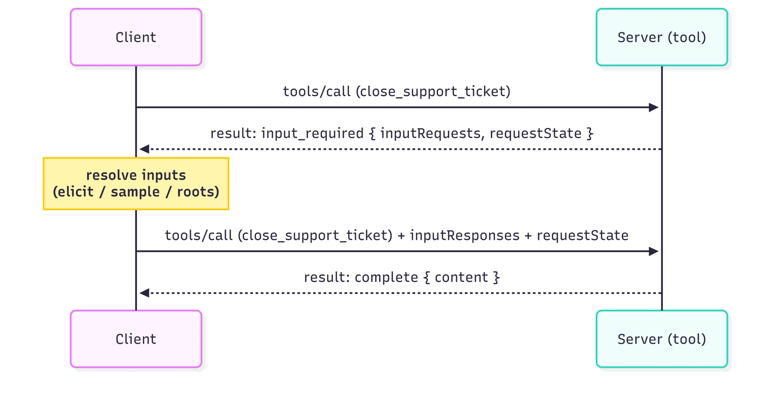
Server support for MRTR
On the server, you throw an InputRequiredException from your tool, passing the inputs you need and a requestState string that will be echoed back to you on the retry. You build the individual requests with the factory methods InputRequest.ForElicitation(...), InputRequest.ForSampling(...), and InputRequest.ForRootsList(...).
Here’s a tool that confirms a significant action before completing it:
[McpServerTool, Description("Closes a support ticket, recording why it was closed.")]
public static string CloseSupportTicket(
    McpServer server,
    RequestContext<CallToolRequestParams> context,
    [Description("The ID of the ticket to close")] long ticketId,
    [Description("Why the ticket is being closed")] string? closeReason = null)
{
    // Handles four client scenarios:
    //  1. Provided up-front: client sends `closeReason` in the initial call
    //  2. MRTR round-trip request: client confirms via `InputResponses["closeReason"]`
    //  3. MRTR initial request: server proposes a default reason and asks for confirmation
    //     (with automatic SDK down-level bridge)
    //  4. Session-less down-level: server returns a guidance message requesting the reason up-front

    // The default reason proposed to the caller and used if none is provided.
    string defaultCloseReason = "completed";

    // (1) Provided up-front. Works on any client, including down-level session-less.
    //     These requests are typically sent after (4) returns a guidance message.
    var confirmedReason = closeReason;

    // (2) MRTR round-trip request. Works with native MRTR support or the automatic down-level
    //     SDK bridge after (3) throws an `InputRequiredException` to request a `closeReason`.
    if (string.IsNullOrWhiteSpace(confirmedReason) &&
        context.Params?.InputResponses?.TryGetValue("closeReason", out var reasonResponse) is true)
    {
        var reasonResult = reasonResponse.Deserialize(InputResponse.ElicitResultJsonTypeInfo);

        // Branch on the elicitation action: `decline` or `cancel` leaves the ticket open.
        if (reasonResult?.IsAccepted is not true) return "Ticket close cancelled";

        // Accepted: use the reason the caller confirmed, falling back to the proposed default.
        confirmedReason = reasonResult.Content?.TryGetValue("closeReason", out var reasonValue) is true
            ? reasonValue.GetString()
            : null;
        confirmedReason = string.IsNullOrWhiteSpace(confirmedReason) ? defaultCloseReason : confirmedReason;
    }

    // (1) or (2) A reason is in hand; proceed with closing the ticket.
    if (!string.IsNullOrWhiteSpace(confirmedReason))
        return $"Closed ticket {ticketId}: {confirmedReason}";

    // (3) MRTR initial request: propose "completed" as the default reason and ask the caller
    //     to confirm (or adjust) it. This uses the 2026-07-28 MRTR input request, but the SDK
    //     provides an automatic bridge to a legacy elicitation on a down-level, stateful
    //     session. When the bridge can be provided, `server.IsMrtrSupported` is `true` and the
    //     exception leads to a legacy elicitation response automatically.
    if (server.IsMrtrSupported)
    {
        throw new InputRequiredException(
            inputRequests: new Dictionary<string, InputRequest>
            {
                ["closeReason"] = InputRequest.ForElicitation(new ElicitRequestParams
                {
                    Message = $"Close ticket '{ticketId}'? Accept the default reason or provide your own.",
                    RequestedSchema = new()
                    {
                        Properties =
                        {
                            ["closeReason"] = new ElicitRequestParams.StringSchema
                            {
                                Title = "Close reason",
                                Description = "The reason for closing the ticket",
                                Default = defaultCloseReason,
                            },
                        },
                    },
                })
            },
            requestState: ticketId.ToString());   // opaque; echoed back to us on the retry
    }

    // (4) Down-level and stateless: we can't prompt an elicitation through an MRTR
    //     round-trip request or an elicitation. Return a natural language response
    //     with guidance for providing the reason up-front.
    return "Closing a ticket requires a reason. Resend with `closeReason`.";
}
One method, every client. The tool can hold a round trip in two situations: a 2026-07-28 client (native MRTR), or a down-level client on a stateful session, where the SDK bridges the same throw to legacy elicitation. In both, it proposes a default close reason and finishes on the retry from context.Params.InputResponses. The one situation it can’t cover is a session-less down-level client, the case that McpServer.IsMrtrSupported rules out. There, it falls back to the closeReason argument, so that caller provides the reason directly instead of being stranded. Same tool, whether the client speaks MRTR or not. The compatibility table below spells out all four cases.
Client support for MRTR
On the client, the high-level McpClient resolves MRTR automatically. Register the matching handlers, and the client will satisfy input requests and re-issue the call for you. You just get the final result back from CallToolAsync.
var client = await McpClient.CreateAsync(
    clientTransport,
    clientOptions: new()
    {
        Handlers = new McpClientHandlers
        {
            ElicitationHandler = (requestParams, ct) =>
            {
                // Accept the proposed default close reason.
                return ValueTask.FromResult(new ElicitResult { Action = "accept" });
            },
        }
    });

// The client transparently handles the input_required round trip.
var result = await client.CallToolAsync(
    "close_support_ticket",
    new Dictionary<string, object?> { ["ticketId"] = 1234L },
    cancellationToken: CancellationToken.None);
One pattern, replacing three
Because MRTR generalizes the “server needs something from the client” interaction, it replaces the previous server-initiated request pattern for elicitation, sampling, and roots on stateless servers.
Elicitation is now achieved with InputRequiredException and InputRequest.ForElicitation(...). The legacy ElicitAsync method continues to work on stateful sessions, but it throws in stateless mode because there’s no session to carry the server-initiated request.
For the special case of secure, out-of-band consent (third-party OAuth, sensitive data), v2 adds UrlElicitationRequiredException for URL-mode elicitation in stateless flows. The client presents a server-hosted URL, gathers consent out of band, and retries. Reference the URL mode elicitation (out-of-band) documentation for more details on this scenario.
Sampling and Roots are deprecated under diagnostic MCP9005 to align with SEP-2577. The SampleAsync and RequestRootsAsync remain available but will also throw in stateless mode.
Logging was also deprecated as part of SEP-2577 due to overlap with stderr and OpenTelemetry. References to those APIs produce warnings with MCP9005.
MRTR and backward compatibility
MRTR is designed to degrade gracefully. Here’s how it behaves across protocol versions and session modes:
| Negotiated protocol | Session mode | MRTR behavior |
|---|---|---|
2026-07-28 |
Stateless | Native: no server-side handler state needed. |
2026-07-28 |
Stateful | Native: InputRequiredResult serialized directly to the wire. |
2025-11-25 and earlier |
Stateful | Back-compat resolver: the SDK bridges to the old session-based requests. |
2025-11-25 and earlier |
Stateless | Not supported: the input request surfaces as an McpException. |
That third row is why the CloseSupportTicket tool above needs no down-level variant: when a v2 server talks to an older client over a stateful session, the SDK automatically bridges MRTR to the old server-initiated request pattern. The fourth row is the only case that can’t be prompted at all (a session-less down-level client), which is exactly why the tool also accepts the optional closeReason argument, giving that caller a non-interactive way through instead of a dead end.
Backward compatible by design
Now let’s pay off the promise from the top of the post. A major version bump can be unnerving, so let’s be specific about what “backward compatible” means here.
Your v1 code keeps working. Stable, non-deprecated 1.x APIs continue to compile and run in 2.0. The deprecations introduced in this release (MCP9005 for the server-initiated requests, MCP9006 for stateful-only options, MCP9004 for legacy SSE) are warnings, not removals. You migrate at your own pace.
Old clients and servers keep working, in both directions. A v2 client transparently uses the legacy initialize handshake when it talks to a down-level server, and a v2 server still accepts that handshake from a down-level client. Upgrading the SDK does not strand you on either side of a connection. This is a deliberate stance the SDK takes: its major versions track spec revisions, but it retains down-level protocol support so a version bump doesn’t force a flag day. Our versioning strategy declared when we released v1.0 remains the same with v2.0.
We’ve been testing this promise in the open. Across the v2 preview releases, adopters confirmed what we most wanted to hear: both the client and the server remain backward compatible with the prior specification revision. A v2 client can drive an older server, and a v2 server can serve an older client, without special handling on your part.
The one honest exception: Tasks
There is exactly one place where v2 is not wire-compatible with v1: the Tasks extension. The redesigned Tasks in 2.0 (SEP-2663) replaces the experimental Tasks from the 2025-11-25 spec extension (supported in v1.3.x and v1.4.x) and is not compatible at the API or protocol level. A v2 client calling a v1 task-server just gets an ordinary tool result, and vice versa. If you adopted the experimental Tasks preview, this is the one migration to plan for. Happily, the new design is much nicer. More on that below.A few migration points:
| v1 | v2 |
|---|---|
| HTTP transport defaults to stateful | Accept the new stateless default, or set Stateless = false explicitly when sessions are required |
Experimental Tasks are built into Core through McpServerOptions.TaskStore and McpClientOptions.TaskStore |
Add ModelContextProtocol.Extensions.Tasks; configure servers with .WithTasks(store) and use CallToolWithPollingAsync or CallToolAsTaskAsync on clients |
Clients start with the initialize handshake |
v2 prefers 2026-07-28 and falls back automatically; pin McpClientOptions.ProtocolVersion only when strict behavior is required |
Packages and target frameworks
One of the quieter but most consequential facts about this SDK is its reach. The v2 packages target net8.0, net9.0, and net10.0, along with netstandard2.0 (for use with .NET Framework).
The packages come in a small, composable set. Start with ModelContextProtocol for most servers; reach for ModelContextProtocol.AspNetCore when you want the Streamable HTTP server; and take just ModelContextProtocol.Core if you only need a client or the low-level building blocks.
| Package | Purpose |
|---|---|
ModelContextProtocol.Core |
Client and low-level server; minimal dependencies |
ModelContextProtocol |
Stdio server, hosting/DI, and attribute-based discovery. Start here |
ModelContextProtocol.AspNetCore |
Streamable HTTP server |
ModelContextProtocol.Extensions.Tasks |
Long-running tools with client polling and pluggable persistence (opt-in) |
ModelContextProtocol.Extensions.Apps |
Interactive, server-delivered UI (experimental; MCPEXP003) |
# Most servers:
dotnet add package ModelContextProtocol

# HTTP servers:
dotnet add package ModelContextProtocol.AspNetCore

# Just a client, or the low-level API:
dotnet add package ModelContextProtocol.Core
The Core package also bundles Roslyn analyzers that catch common mistakes at build time, so a lot of the guidance in this post is enforced right in your editor.
Extensions: Apps and Tasks
You may have noticed two packages in that table that aren’t part of the base SDK: ModelContextProtocol.Extensions.Apps and ModelContextProtocol.Extensions.Tasks. That’s not an accident of packaging. It’s the architecture.
The 2026-07-28 revision makes extensions a first-class concept, negotiated through capabilities beyond the core protocol. The MCP C# SDK leans all the way into that idea: Apps and Tasks are not baked into the base SDK. They ship as separate packages that bolt onto ModelContextProtocol.Core, and they’re strictly opt-in. You add them only when you want them, and the base SDK stays lean. It’s the same “pay as you go” principle as statelessness: take a dependency only on what you use.
- MCP Apps lets servers deliver interactive UIs inside supporting clients (SEP-1865). You enable it with
.WithMcpApps()and annotate tools that provide UI resources. MCP Apps are experimental and the APIs require suppressing diagnosticMCPEXP003. - Tasks supports long-running tool execution with client-side polling and pluggable persistence (SEP-2663). You can get started with
.WithTasks(new InMemoryMcpTaskStore()), and MRTR flows through the task store so long-running tools can ask for input too.InMemoryMcpTaskStoreis intended for development and testing; for tasks that must survive process restarts or work across server instances, implementIMcpTaskStoreusing durable shared storage.
MCP Apps and Tasks each deserve posts of their own, but for now the point is architectural: the SDK is deliberately built so these capabilities are add-ons you opt into. As MCP concepts continue to emerge and evolve, we are striving to keep the ModelContextProtocol and ModelContextProtocol.Core packages lean and limited to behaviors baked into the base protocol.
What’s next
With the 2026-07-28 spec compliance landing in 2.0, the SDK’s next focus is end-to-end authentication and authorization: making secure MCP deployments as turnkey as the rest of the stack, building on the closer OAuth and OpenID Connect alignment the spec introduced. That work continues in the 2.x line, and you can follow it in the open.
Summary
The 2.0 release of the MCP C# SDK is a milestone for building MCP servers and clients on .NET. MCP has grown up for the web (stateless by default, routable by ordinary infrastructure, and interactive without sessions thanks to Multi Round-Trip Requests), and .NET is ready for it, riding on ASP.NET Core and reaching all the way back to .NET Framework. Best of all, you get there without leaving your existing clients, servers, or code behind.
If you’re building MCP servers or clients in .NET, now is a great time to upgrade.
Have a question, a bug, or an idea? The best place to reach the team is the csharp-sdk repository: open an issue or start a discussion, and take a moment to skim the 2026-07-28 specification changelog for the full list of what changed in the MCP protocol specification. When you’re ready to explore further, the packages and the full 2.0.0 release notes are the place to start. We can’t wait to see what you build.
The post Announcing v2.0 of the official MCP C# SDK appeared first on .NET Blog.
Pennsylvania, USA
Anytime a new version of something comes out in the tech industry—LLMs, mobile phones, services—people start asking “what’s next” a moment later. I’m quite excited by all the stuff in our Google queue, but I’m more interested in what’s already shipped. Let’s use what we got before obsessing over things we don’t have.
[blog] How AI Is Changing Open Source. More (random) projects, overwhelmed maintainers, and declining motivation to go to the effort of open sourcing? Sounds dire. Still reason for optimism.
[blog] Rich UI in Gemini Enterprise: A Field Report on A2A Agents and A2UI Primitives. Is the future of software distributed agents that use dynamic UIs for user interaction? Possibly. Pay attention to generative UI developments.
[article] MCP’s biggest update removes the machinery many servers were built around. A remote MCP server can now act more like a stateless HTTP service. This will require some changes, but should simplify things for many. More here, and here.
[blog] Don’t Let Your Agent Mess Up Your Database. Speaking of MCP, this is a great solution to a missing feature of MCP.
[blog] 3 things top 1% teams do differently. Your mileage may vary, but this post says that improving hiring, embracing parallelization, and adapting your code review flow are keys to success.
[blog] Detect early and enforce firmly with Google Cloud’s enhanced cost controls for AI spend. We’re doing some good work to try and get you ahead of any runaway costs.
[blog] How I set up containerized dev environments you can spin up in seconds for Antigravity CLI, Neat project. Isolate an agentic CLI into its own sandbox so that you can give it a limited set of rights before letting it go wild.
[article] Friday Forward – Be Bored. Big fan of forced boredom. Especially for adults. Sit still. Just be. Give your brain a chance to make novel connections.
[blog] Gemini API Managed Agents: 3.6 Flash, hooks, and more. Sweet update. Define your custom agent (prompt, tools, whatever) and have it run on a schedule in the cloud.
[article] Our Favorite Management Tips on Setting Strategy When the Path Is Unclear. I liked these. Few of us work in boring, stable places. Are you effectively navigating the constant change?
[blog] Merge Conflicts Are a Process Problem, Not a Git Problem. A merge conflict happens when Git doesn’t know which change should win. That’s a team problem to fix.
[article] Why I write skills instead of agents for knowledge work. Don’t customize an agent or LLM when a skill will do. Karl outlines his current thinking.
[article] Enterprises contend with mounting AI costs as tools sprawl. Not surprising. We’re in the experimentation stage where you’ve got to try a mix of tools before you consolidate. This post links to a series of articles on the topic.
[blog] Vibe code your first Android app with Antigravity 2.0 & Android Studio. Wow, Alicia made this workflow actually feel approachable. I may try it myself.
[blog] Google Cloud Skills Tutorial — Part 4 : Google Cloud Solution Architecture Skill. This scenario is exactly why agent skills are useful. Instead of relying solely on what an LLM knows (or what a search agent can scrape), feed your harness a skill that steers it to the most relevant cloud architecture.
Want to get this update sent to you every day? Subscribe to my RSS feed or subscribe via email below:

Pennsylvania, USA
Next Page of Stories