While we copy and invoke the delegate only from its original context, we still destruct it from a possibly-wrong context.
This is a serious problem not just because the non-agile delegate might not be using thread-safe atomic instructions to manage its reference count, but even worse, if the release drops the reference count to zero, the delegate will destruct on the wrong thread, and that will probably create lots of problems.
We have to destruct the non-agile delegate in its original context. We can do this with a std::unique_ptr and a custom deleter. The std::unique_ptr handles all the move operations and the deleter cleans up the last pointer.
This stateful deleter remembers the context to use for final destruction. When it’s time to do the destruction, we switch into the target context via IContextCallback::ContextCallback and take ownership of the raw pointer into a winrt::IUnknown. The destructor of the winrt::IUnknown will perform the release.
We can use this stateful deleter around the raw delegate pointer.
// Don't use this yet - read to the end of the series
template<typename Delegate>
std::remove_reference_t<Delegate> make_agile_delegate(Delegate&& d)
{
if (d.try_as<::IAgileObject>()) {
return d;
}
if (d.try_as<::INoMarshal>()) {
void* p; if constexpr (std::is_reference_v<Delegate>) { p = winrt::detach_abi(d); } else { winrt::copy_to_abi(d, p); }
return
[p = std::unique_ptr<void, in_context_deleter>(p),/* context = winrt::capture<IContextCallback>(CoGetObjectContext), */
token = get_context_token()](auto&&...args) {
if (token == get_context_token()) {
std::remove_reference_t<Delegate> d;
winrt::copy_from_abi(d, p.get());
d(std::forward<decltype(args)>(args)...);
} else {
throw winrt::hresult_error(CO_E_NOT_SUPPORTED);
}
};
} else {
return [agile = winrt::agile_ref(d)](auto&&...args) {
return agile.get()(std::forward<decltype(args)>(args)...);
};
}
}
The first block gets a raw ABI pointer, either by moving it out of the inbound delegate if we can, else by copying it from the inbound delegate.
The second part wraps the raw ABI pointer inside a std::unique_ptr with our custom deleter, and the custom deleter makes sure that the Release of the original delegate happens in the correct context.
In the modern data landscape, most of the effort doesn’t go into building models or dashboards. It goes into getting the data into a usable state. Generally, a large portion of time is spent extracting, cleaning, and reshaping data before any analysis can begin. While Python and SQL together form a powerful stack, the boundary between them is often where things start to break down.
In this article, you’ll learn how to build a more reliable flow by pushing the right work into SQL and keeping Python focused on what it does best: analysis. Plus, expert tips and advice on views, CTEs, pruning, and efficient data extraction.
The foundation: establishing the ‘contract’ layer
A robust pipeline requires an abstraction layer that shields downstream scripts from underlying database fragility.
Views as analytical contracts
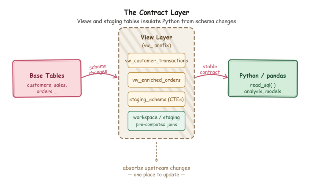
One of the most underused patterns in data engineering is database views, specifically as a stable contract between SQL schema and Python. When we write queries directly against base tables, the Python scripts inherit every structural assumption baked into those tables. A renamed column, a modified join, or a schema migration can silently break downstream logic.
The practical fix involves introducing a dedicated view layer – typically prefixed with vw_ – that the Python code can query instead. These views absorb upstream schema changes. By updating the view definition in just one place, everything downstream can continue to function without modification when an underlying table evolves. Effectively, the view becomes the agreed-upon representation of the data rather than just a passthrough.
CREATE VIEW vw_customer_transactions AS
SELECT
    c.customer_id,
    ...
    s.sales_transaction_date,
    ...
FROM customers c
INNER JOIN sales s ON c.customer_id = s.customer_id
WHERE s.sales_transaction_date >= '2025-07-01';
For Python’s script, the underlying tables don’t really exist. The script only interacts with vw_customer_transactions. Without this layer, analytical logic such as joins and filters tend to leak into Python and become redefined across multiple scripts.
The workspace schema explained
For multi-step or computation-heavy transformations, relying on on-the-fly joins inside extraction queries is inefficient and difficult to maintain. Instead, introduce a ‘workspace schema’ dedicated to intermediate analytical work. This way, pre-computations are isolated into a controlled namespace rather than cluttering the primary schema with temporary logic. This makes it immediately clear which objects are ephemeral and keeps the catalog clean.
In SQL Server, this can be implemented using schema-qualified staging tables (or GlobalTempTables) for cross-session visibility. The idea is simple: compute expensive joins once, then reuse the result.
Consider a churn prediction dataset where relevant features span multiple tables. Recomputing joins every time a feature changes is wasteful. Instead:
-- Pre-compute the heavy join once per session
CREATE TEMP TABLE staging_enriched_orders AS (
    SELECT
        o.order_id,
        o.customer_id,
        p.category AS product_category,
        ...
    FROM orders o
    JOIN products p ON o.product_id = p.product_id
    LEFT JOIN regions r ON o.region_id = r.region_id
);

-- Lightweight extraction
SELECT * FROM staging_enriched_orders
WHERE product_category = 'Electronics'
  AND order_date >= '2026-01-01';
During iterative development, this approach avoids repeatedly paying the cost of complex joins. You compute just once per session, so subsequent extractions become lightweight and fast.
Explaining logical abstraction with common table expressions (CTEs)
As SQL queries grow, deeply nested logic quickly becomes unreadable and fragile. Common Table Expressions (CTEs) provide a way to modularize SQL logic, much like functions do in application code. Using the WITH clause, we define named intermediate steps that isolate distinct parts of the transformation.
Instead of a monolithic query, build a sequence of logical steps that are easier to read, debug and modify. CTEs act as a structural guide through complex transformations, ensuring that by the time data reaches Python, its lineage and logic are already clear.
The contract layer
Fast, reliable and consistent SQL Server development…
…with SQL Toolbelt Essentials. 10 ingeniously simple tools for accelerating development, reducing risk, and standardizing workflows.
The database should act as a strict bouncer. This is to ensure that only pristine, necessary data is allowed into the memory buffer.
Dimensional pruning explained
The first rule of data extraction is simple: don’t pull what you don’t need. Yet, in practice, SELECT * still shows up in production pipelines far too often.
Vertical pruning (projection pushdown) means only selecting the columns your downstream logic actually requires. If a table has 40 columns and you use 8, for example, the remaining 32 columns represent unnecessary network transfer, deserialization, and memory usage.
Horizontal pruning (predicate pushdown) means applying filters as early as possible using WHERE clauses. When filtering happens in SQL, the database engine can leverage indexes and eliminate rows before they’re transmitted. When filtering happens in Python, the cost has already been incurred.
String sanitization explained
Text data is often inconsistent and can create significant downstream issues. Cleaning strings at the database level avoids unnecessary work in Python and ensures consistency across all consumers.
For example: TRIM(LOWER(email)) standardizes casing and removes whitespace before the data ever leaves the database. The equivalent in Pandas, df['email'].str.strip().str.lower(), does work, but only after the data has already been transferred and loaded into memory.
More importantly, normalization at the source ensures correctness. If two records differ only by casing (e.g User@Example.com vs user@example.com), they will not join correctly unless standardized. Handling this in SQL guarantees consistency regardless of which script consumes the data.
Strict type enforcement
Python’s performance model depends on consistent, predictable data types, especially when working with Pandas or NumPy. Weak or implicit typing at the SQL layer often leads to subtle downstream issues that are difficult to debug.
An example is SQL Server’s BIT type being interpreted inconsistently in Python, sometimes appearing as integers (0/1) instead of boolean values. Similarly, numeric fields may be inferred as object types if NULL values are present, which breaks vectorized operations and slows computation.
The fix is to enforce type consistency at the source. Using explicit casting ensures that the data arrives in Python exactly as expected:
CAST(is_active AS BIT) AS is_active_flag,
CAST(total_amount AS FLOAT) AS total_amount,
CAST(order_date AS DATETIME2)COALESCE(discount_amount, 0) AS
discount_amountAS order_timestamp
Equally important is handling missing values proactively. Leaving NULL values unmanaged often results in unintended NaN propagation in Pandas, which can silently alter aggregations or model inputs.
COALESCE(discount_amount, 0) AS discount_amount
Once data enters Python, type inconsistencies become exponentially harder to trace because they manifest during transformations rather than at ingestion.
The engine: leveraging set-based logic to eliminate heavy Python compute
Relational databases are highly optimized for set-based logic. Offloading the compute to the database engine saves massive amounts of CPU overhead in Python.
Temporal alignment with window functions
Time-series analysis in Python often involves operations like computing the previous value, calculating rolling averages, or ranking records within groups. The typical approach is to extract raw data and apply Pandas shift(), rolling(), or groupby().rank(). Window functions allow you to push this entire class of computation into the database engine, where it can be executed more efficiently as part of a set-based query.
Consider a scenario where a team needs to analyze a sudden 20% drop in pre-orders for a product. A naive approach would involve pulling daily sales into Python and computing week-over-week changes. The better solution is to compute this directly in SQL:
SELECT
    sales_date,
    SUM(sales_amount) AS daily_sales,
    LAG(SUM(sales_amount), 7) OVER (ORDER BY sales_date) AS sales_7_days_ago,
    SUM(sales_amount) - LAG(SUM(sales_amount), 7) OVER (ORDER BY sales_date) AS weekly_delta
FROM sales
GROUP BY sales_date
ORDER BY sales_date;
Here, the database aggregates, aligns temporal context and computes comparative metrics all before the data ever reaches Python. The result is a time-series dataset usable for analysis or modeling.
Statistical pre-processing explained
Databases natively support statistical functions like standard deviation, variance and percentile ranks, etc. When the goal is to prepare data for modeling rather than explore it interactively, computing these metrics in SQL is often more efficient.
This also applies to A/B testing workflows. Rather than extracting raw event-level data, you can compute per-group aggregates, counts, means and variances directly in SQL. Then, you can send a compact summary to Python for hypothesis testing. The result is less data movement and a clearer separation of responsibilities between systems.
Complex data flattening explained
Modern schemas often include semi-structured data such as JSON, arrays, or nested attributes. Parsing these structures in Python introduces unnecessary overhead and typically results in row-by-row processing, which is slow and difficult to maintain. SQL, on the other hand, provides native operators for working with these types.
SELECT
    event_id,
    user_id,
    event_timestamp,
    event_data ->> 'event_type' AS event_type,
    event_data ->> 'page_url' AS page_url,
    (event_data ->> 'session_duration_seconds')::INTEGER AS session_duration,
    JSONB_ARRAY_LENGTH(event_data -> 'items_viewed') AS items_viewed_count,
    event_data -> 'items_viewed' -> 0 ->> 'product_id' AS first_item_viewed
FROM user_events
WHERE event_timestamp >= NOW() - INTERVAL '30 days'
  AND event_data @> '{"event_type": "page_view"}';
This produces a flat, tabular dataset without navigating nested structures in Python.
The extraction: performance and throughput
When the data is clean and flattened, the physical transfer method dictates the speed of pipeline.
Vectorized transfers explained
Traditional row-by-row cursors like standard psycopg2 (or similar adaptors) introduce significant overhead, because each row is deserialized individually. Modern data pipelines favor columnar, vectorized transfers, often using Apache Arrow as the underlying format.
Libraries like Polars, combined with high-performance connectors such as ConnectorX, allow data to be loaded directly into memory in a columnar layout. This significantly improves throughput and reduces CPU overhead for enterprise scale. In practice, this can reduce extraction times dramatically without changing the SQL query itself.
Extraction strategy selection
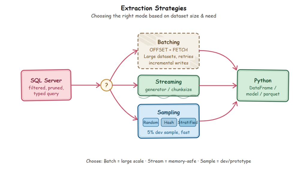
The optimal extraction strategy in databases depends on data size and processing requirements. Batching, for example, splits large datasets into manageable chunks using OFFSET and FETCH. This means repeatedly querying ordered slices of data (e.g., ORDER BY order_id LIMIT n OFFSET k), which supports incremental writes, retrying failed batches, and progress tracking. However, large offsets can degrade performance.
An alternative is Streaming, which avoids this issue by consuming results incrementally using Python generators and chunked reads (chunksize) from a single query. It yields values one at a time rather than returning everything at once. Memory usage remains stable because only one chunk is processed at a time. This is the preferred approach when processing is sequential and doesn’t require random access.
Stratification and sampling
When prototyping machine learning models or testing pipeline logic, analyzing the entire ‘Big Data’ warehouse is counterproductive and wastes expensive compute resources. A smaller, representative subset is enough – plus, it’s significantly faster to iterate on. There are three distinct sampling strategies, each serving a different purpose:
Random sampling is the simplest approach. Most databases support this directly through constructs like TABLESAMPLE (n PERCENT), which returns an approximate fraction of rows. It’s fast and easy to use, but not reproducible.
For reproducibility matters such as debugging or consistent experimentation, deterministic sampling is more reliable. This is typically done by hashing a stable identifier (e.g., HASHTEXT(customer_id)). Because the hash output is consistent, the same subset of records is selected every time.
Stratified sampling is used when the dataset is imbalanced. Instead of sampling globally, the data is partitioned into groups (e.g., PARTITION BY is_fraud) and sampling is applied within each group. This is commonly implemented using window functions like ROW_NUMBER() to select a proportional subset from each category. This ensures that both majority and minority classes are preserved in the final sample.
Consider fraud detection, where fraudulent transactions might represent only 0.3% of total data. A naive random sample may include too few fraud cases to be useful. Stratified sampling ensures that each subgroup is proportionally represented.
WITH fraud_sample AS (
    SELECT *, ROW_NUMBER() OVER (
        PARTITION BY is_fraud
        ORDER BY HASHTEXT(transaction_id::TEXT)
    ) AS rn,
    COUNT(*) OVER (PARTITION BY is_fraud) AS stratum_total
    FROM transactions
    WHERE transaction_date >= '2025-01-01'
)
SELECT
    transaction_id,
    Is_fraud,
    ... -- relevant features
FROM fraud_sample
WHERE rn <= stratum_total * 0.05;
Extraction strategies
Putting it all together
Across all these patterns, the principle remains consistent. SQL databases are optimized for transformation, filtering, and aggregation. Python is optimized for modeling, statistical analysis, and application logic.
The extraction layer is where responsibility shifts from one system to the other. When this boundary is designed deliberately using contracts, pruning, pre-computation, and efficient transfer mechanisms, you spend less time maintaining pipelines and more time doing meaningful analysis.
None of these ideas are individually complex. The difference comes from applying them intentionally, rather than defaulting into patterns that seem convenient in the moment but fail under scale.
References
Shan, J., Goldwasser, M., Malik, U., & Johnston, B. (2022). SQL for data analytics (3rd ed.)
Illinghton, A. (2024). Python programming and SQL: 6 books in 1
Simple Talk is brought to you by Redgate Software
Take control of your databases with the trusted Database DevOps solutions provider. Automate with confidence, scale securely, and unlock growth through AI.
FAQs: How to get clean, usable data out of SQL Server into Python
1. Why should data transformations be pushed into SQL instead of Python?
SQL engines are optimized for set-based operations like filtering, joining, and aggregation. Performing these tasks in SQL reduces data transfer, improves performance, and simplifies Python code.
2. What is a “contract layer” in data pipelines?
A contract layer (often implemented with database views) acts as a stable interface between raw tables and downstream code, protecting pipelines from schema changes.:
3. How do database views improve pipeline reliability?
Views abstract underlying schema complexity. When base tables change, only the view needs updating—downstream Python scripts remain unaffected.
4. What is dimensional pruning and why does it matter?
Dimensional pruning means selecting only required columns (vertical) and rows (horizontal). This reduces memory usage, speeds up queries, and minimizes unnecessary data transfer.
5. Why should data cleaning (e.g., string normalization) happen in SQL?
Cleaning data at the source ensures consistency across all consumers and avoids redundant processing in Python after data is loaded.
6. What are Common Table Expressions (CTEs) used for?
CTEs modularize complex SQL queries into readable steps, making transformations easier to debug, maintain, and extend.
7. When should you use a workspace or staging schema?
Use it for heavy joins or intermediate computations that are reused multiple times, improving performance and keeping production schemas clean.
8. How do window functions improve performance?
Window functions handle time-based calculations (like rolling averages or lag comparisons) directly in SQL, eliminating the need for expensive Python computations.
9. What is the best way to extract large datasets efficiently?
Use vectorized, columnar transfers (e.g., Apache Arrow-based tools) or streaming approaches instead of row-by-row extraction to improve speed and reduce memory usage.
10. What sampling strategies are best for large datasets?
Random sampling for quick exploration
Deterministic sampling for reproducibility
Stratified sampling for imbalanced datasets (e.g., fraud detection)
TL;DR: CSV exports slow down modern web apps with version issues, stale data, and broken validation. In-browser spreadsheets offer a more efficient approach by enabling structured, real-time editing directly inside applications, improving data consistency, user experience, and workflow efficiency across dashboards, operations, and internal tools.
If your app still relies on “Export to CSV” for quick edits, you’ve probably seen this happen:
Someone downloads a file, opens it in Excel or Google Sheets, makes a few updates… and then things start getting messy.
Which version is the latest?
Why did the upload fail?
Who changed this value?
At first, it feels like a simple workflow. But once teams depend on it daily, the cracks start to show.
A modern alternative is an in-browser spreadsheet: an Excel-like editor embedded directly in your web app. Users edit data in place with familiar spreadsheet interactions without leaving the product.
In this article, we’ll look at how to embed an in-browser spreadsheet in React using Syncfusion®React Spreadsheet Editor.
The hidden problem with CSV exports
CSV exports weren’t designed for continuous, in-app data editing. They were a workaround useful at a time when web apps couldn’t handle complex grids.
Today, that workaround creates more problems than it solves.
Here’s what typically goes wrong:
Version confusion: Multiple files floating around, no clear “source of truth”.
Stale data: The moment a file is exported, it starts drifting away from live data.
Broken structure: No formulas, no formatting, no validation, just raw values.
Individually, these are small issues. Together, they slow teams down and introduce unnecessary risk.
When the export breaks, productivity follows
What looks like a simple loop export, edit, and upload quietly adds friction at every step.
Now imagine a finance team updating quarterly forecasts.
They export a CSV, tweak some numbers, and re-upload it. But formulas are gone, number formats are inconsistent, and validation rules don’t exist anymore.
Someone spots an error. Another file is downloaded. Another version is created.
By the time data is “final,” nobody fully trusts it.
This isn’t a tooling issue; it’s a workflow problem.
So what’s changing?
Instead of pushing users out to Excel, many modern web apps are doing the opposite:
They’re bringing spreadsheet-like editing directly into the application.
This means:
Edit data in place
Keep everything connected to live data
Apply validation before errors happen
Maintain a single source of truth
No exports. No uploads. No guesswork.
CSV exports vs. in-browser Spreadsheets: What actually changes
Here’s the real difference, not in features, but in experience:
CSV Workflow
In-Browser Spreadsheet
Download → Edit → Upload
Edit instantly inside the app.
Static snapshot of data
Always working with live data.
No built-in validation
Controlled, rule-based editing
Multiple file versions
One shared source of truth.
Error-prone updates
Guided, structured changes
The shift isn’t just technical; it’s about removing unnecessary steps.
When CSV still makes sense
CSV exports still have their place.
They’re useful when:
Data needs to be shared externally
Offline access is required
The task involves one-time exports
The problem arises when CSV becomes the default for everyday editing.
What makes an in-browser Spreadsheet enterprise-ready?
Embedding a spreadsheet into a production application requires more than just rendering a grid.
Key considerations include:
Performance: Large datasets need efficient rendering (virtualization) and a careful recalculation strategy.
Scalability: Define how edits sync to your backend (save-on-change vs save-on-submit, conflict handling).
Maintainability: Prefer a component with stable APIs and documented configuration patterns.
Security/permissions: Restrict editing by role, protecting sheets/ranges, and validating inputs at the cell level.
Accessibility: Keyboard navigation and screen reader support matter for enterprise rollouts.
The modern approach: In-browser Spreadsheet Editor
An embedded spreadsheet component brings spreadsheet-style editing directly into your web app, without forcing users to switch tools.
Instead of exporting files and re-importing them later, users can work with data in a structured, interactive grid that stays connected to your application.
This approach allows your app to stay in control of:
Data access and permissions
Validation and business rules
Real-time updates and consistency
Today, many teams use ready-made spreadsheet components to support this pattern, rather than building everything from scratch.
For example, in a React application, a component like the Syncfusion React Spreadsheet Editor can provide the core functionality needed to support in-app editing, including handling large datasets, applying validation, and maintaining a consistent data structure.
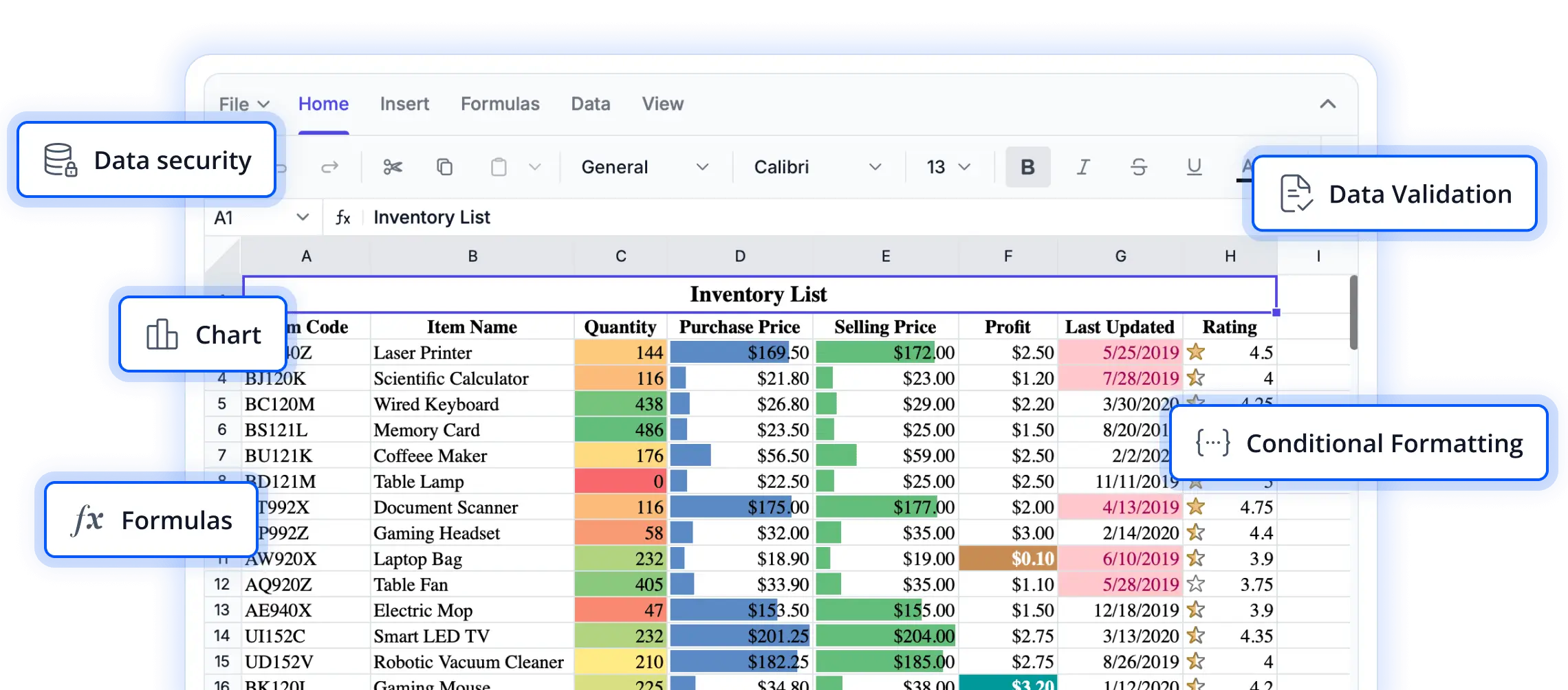
Advanced data management features in React Spreadsheet
Embedding an In-Browser Spreadsheet in a React app
Instead of relying on exports, you can bring spreadsheet-style editing directly into your React application with a ready-to-use component.
At a high level, the integration is straightforward. Once the spreadsheet component is added to your project, it can render an interactive grid in your app, allowing users to start editing data immediately. From a user’s perspective, this feels very similar to working in Excel or Google Sheets, but without leaving the application.
In a typical setup, you import the spreadsheet component into your React app and render it like any other UI element:
import * as React from 'react';
import { SpreadsheetComponent } from '@syncfusion/ej2-react-spreadsheet';
import './App.css';
export default function App() {
    return  (<SpreadsheetComponent/>);
}
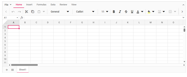
React Spreadsheet Editor
From there, you can layer in additional capabilities based on your use case, whether that’s loading data, applying validation rules, or enabling formatting and formulas.
Rather than building complex grid logic from scratch, this approach lets you focus on how users interact with data in your product, while the spreadsheet component handles the heavy lifting behind the scenes.
If you want to go deeper into configuration and advanced capabilities, the official documentation covers everything from data binding to feature customization.
Real-world scenarios where it makes a difference
This approach becomes especially valuable in workflows where data changes frequently:
Internal dashboards and admin tools: Teams can update operational data directly, without switching tools or managing multiple file versions.
Finance and operations: Maintaining structured data helps reduce errors in calculations and reporting.
HR and large datasets: Managing large volumes of structured data becomes more reliable and easier to navigate.
Sales and pricing tools: Teams can quickly test scenarios and update values without interrupting their workflow.
Data entry portals: Built-in validation ensures cleaner, more consistent data from the start.
These aren’t edge cases; they reflect how many teams already work today.
Frequently Asked Questions
Will an in-browser spreadsheet work with existing Excel files?
Yes. You can open and export Excel (XLSX) and CSV files directly in the browser. Most formatting, formulas, and structure are preserved, so you don’t lose context when working with existing files.
Can an in-browser spreadsheet edit CSV files directly?
Yes. CSV files can be opened, edited, and validated within the spreadsheet interface, and then exported again if needed.
What features does an in-browser spreadsheet provide?
Can an in-browser spreadsheet control what users are allowed to edit?
Yes. You can restrict access using sheet protection, locked ranges, and validation rules, along with your application’s permission system.
Does an in-browser spreadsheet support accessibility and localization?
Yes. It includes keyboard navigation, screen reader support (WAI-ARIA), RTL layouts, and localization for dates and formats, making it suitable for global applications.
Final thoughts
Many web apps still rely on CSV exports because “that’s how it’s always been done.”
But the reality is, teams are quietly moving away from it, especially in products where data changes frequently.
If your users are exporting files every day just to make edits, it’s worth asking: Is the process helping them, or slowing them down?
Because sometimes, the biggest improvement isn’t a new feature, it’s removing an unnecessary step.
For React teams, our React Spreadsheet Editor provides a practical path to deliver an Excel-like experience with import/export and performance features. If your users edit data every day, it’s worth evaluating an embedded spreadsheet approach and testing it against your current CSV workflow.
Still depending on CSV files for daily workflows? Switch to a modern in-browser spreadsheet and see the difference yourself with the live demo.
If you’re a Syncfusion user, you can download the setup from the license and downloads page. Otherwise, you can download a free 30-day trial.
In the 2010s, if you had technical gaps (say, you couldn’t write CSS), you had to either rely on a skilled colleague or just hope that the answer to your exact problem was out there on the internet. Today, everyone can write sort-of-okay CSS by delegating the task to an LLM. LLMs make everybody into a generalist.
Because of this, lots of people don’t think there’s any skill involved in working with LLMs. If you want the product that LLMs can deliver — PhD-level mathematics, pretty good but sometimes tasteless computer code, or awkward LinkedIn-style writing — you can simply ask for it. Since everyone is talking to the same models, “skilled prompters” are getting the same results as people touching LLMs for the first time.
This is wrong. The most important skill in prompting is expertise in the domain you’re prompting for.
A good illustration of this is Terence Tao’sconversation with ChatGPT about the recently-discovered counterexample to the Jacobian Conjecture. This is not the same ChatGPT I talk to! I couldn’t get to where Tao gets, even with unlimited tokens to burn.
There’s a lot to learn about good prompting from Tao’s conversation. Here are a few observations:
Tao’s messages are very short and to-the-point. He doesn’t respond point-by-point to the model, just to the gist
The model outputs are much more concise than when I try and talk to GPT-5.6 Sol about mathematics. By signalling expertise, Tao shunts the model into “talking-to-mathematicians” mode, not “explaining-to-amateurs” mode
Tao pushes back when the model’s responses look wrong, but he doesn’t directly contradict; instead, he says things like “this looks more complex than I was hoping for”
Tao makes several leaps and suggestions himself. He almost never takes the model’s advice about where to go next
However, you can’t prompt like Tao on mathematical questions just by following these tips. The key to his technique is actually understanding the mathematics: pulling the relevant idea out of ChatGPT’s multi-paragraph response, suggesting alternate approaches or formulations, and identifying what “looks weird”.
Terence Tao is a better mathematician than I am a programmer. But the idea here — that domain knowledge makes you better at using LLMs — is something I’ve also experienced in my own work. If you have a good theory of your codebase, you can push the LLM much harder than if you have no familiarity. Because you have your own sense of what a good solution might look like, you can say “no, I think it could be simpler here”, or “but don’t we already do X?”, or “can we express this problem in these familiar terms?“.
This touches on an idea I’ve written about before: that system design problems are dominated by concrete specifics, not generic principles. Of course both are useful, but I’d rather have familiarity with the codebase than a deep general understanding of software systems. In his conversation, Terence Tao asks a lot of specific questions like “does X work here?”, or “given Y and Z, why A?“. I can’t ask those questions about the Jacobian Conjecture, but I can ask them about the systems I own at GitHub.
If you have no domain knowledge, you can cling onto the LLM to at least get something. That’s not bad! But if you have domain knowledge, you can wring far more value out of the same LLM by steering it hard in the direction you want. Most of us will have to do a mix of both these approaches, since we have domain knowledge in some areas but not others.
The usefulness of domain knowledge suggests that human expertise will continue to be useful even as models get stronger. For many tasks, the human is the bottleneck, not the model, because the difficult part is in communicating to the model exactly what kind of solution the human wants. The information is “in the model” already, but it takes a very smart human to pull it out.
Meet Darling: Free, Headless Fleet Performance Monitoring for SQL Server
Watching one SQL Server is easy. Watching fifty is where monitoring vendors smell blood. The price is per server, per year, and it climbs every time your environment grows. Your reward for paying it: your performance data gets shipped to somebody else’s cloud, where you look at it through dashboards built by people who’ve never tuned a query in their lives.
Darling is my answer to that. It’s the new flagship edition of my free, open source SQL Server Performance Monitor. One SQL Server or five hundred, one product, no per-server tax, and your data never leaves your network.
What Darling is
Darling is a headless Windows service. You install it on one monitoring host, point it at your servers, and it collects around the clock. Nobody has to be logged in. Nothing gets installed on the monitored servers for its own storage.
It brings its own database. The installer bootstraps a managed PostgreSQL instance with TimescaleDB and runs it for you. There’s no repository server to stand up, no schema to deploy, no extra license to buy. Darling replaces the old SQL-Server-backed Dashboard edition, which needed a SQL Server of its own to store what it collected.
What it collects
36 collectors, the same shared library Lite uses: wait stats, query stats from the plan cache, Query Store, active query snapshots, blocking, deadlock graphs, execution plans, tempdb, memory grants and clerks, file IO latency, CPU, Agent jobs, server configuration, and more. Deltas are computed for you, so you see the work done between snapshots instead of staring at cumulative counters.
The store is yours
Everything lands in a PostgreSQL store you own. Not an API. Not an export wizard. Not a vendor data lake. Point any SQL client at it and query.
— Top waits across the fleet, last 24 hours SELECT server_name, wait_type, sum(wait_time_ms) AS total_ms FROM collect.wait_stats WHERE collection_time >= now() – interval ‘1 day’ GROUP BY server_name, wait_type ORDER BY total_ms DESCLIMIT 10;
Views are included for the common questions, but you’re not limited to them. It’s just tables. Join them however you want, feed Power BI, export to Excel.
Alerts without a babysitter
A real-time alert engine runs continuously: blocking, deadlocks, poison waits, long-running queries, tempdb space, long-running Agent jobs, high CPU, and servers that stop answering. Since Darling is headless, alerts go out by email and webhook (Slack, Teams, or any endpoint you point it at). Emails carry the query text, blocking chains, and deadlock XML. When a condition clears, it tells you that too. For the alerts that cry wolf, there are mute rules by server, metric, database, query, wait type, or job, with optional expiration.
An MCP server that can do things
Both editions ship a built-in MCP server, so an AI assistant like Claude can read your performance data directly. Darling’s can also write. An agent can build Custom Views, tune alert thresholds and mute rules, and onboard an entire fleet, all over MCP. Standing up monitoring for twenty servers is a sentence, not an afternoon.
Watch it from a browser
An optional read-only web dashboard shows the fleet from any browser, no install. It’s off by default and binds loopback-only until you deliberately expose it, token-gated and scoped to the network range you allow.
Custom Views and notebooks
This is the part the desktop app never had. Compose your own views over the collected data: pick the metrics, filters, grouping, and charts, or build notebook pages that mix charts with commentary. Make them by hand, or have an AI make them for you over MCP.
How to get it
Download the Darling zip, run the scripted install from an elevated prompt, and it bootstraps the Postgres store and starts the service. Add servers by pasting a list into the viewer, or over MCP. SQL Server 2016 through 2025, Azure SQL Managed Instance, Azure SQL Database, and AWS RDS are supported. Every release is signed.
There’s no paid version, and no locked features. If your compliance team needs a vendor agreement and a support contact on file before anything touches production, there’s a support subscription for that. The software is identical either way.
And Lite is not going anywhere
Lite, the desktop app with its local DuckDB store, is still here and still supported. Same 36 collectors, same shared brain. Darling is the answer for fleets and headless monitoring. Lite is the answer for the one machine you’re sitting in front of. Pick the one that matches your day.
Going Further
If this is the kind of SQL Server stuff you love learning about, you’ll love my training. Blog readers get 25% off the Everything Bundle — over 100 hours of performance tuning content. Need hands-on help? I offer consulting engagements from targeted investigations to ongoing retainers. Want a quick sanity check before committing to a full engagement? Schedule a call — no commitment required.
 Log in